问题分析
问题发现
通过对蘑菇的外观特征进行识别,从而判断蘑菇是否可食用,是从我们从古至今依然在使用的方法,我国云南省等地仍然有着吃野菌菇的习惯,尽管人们已经总结了许多识别野菌菇的方法,比如颜色、褶皱、菌盖的大小等等,但是在每年在云南仍然有大量的因食用有毒的野蘑菇而中毒致幻的受害者,因此仅仅根据人工总结出的,比较单一结构进行评判的经验,并不能保证对蘑菇进行分类的准确性。
因此考虑使用机器学习的方法来解决蘑菇分类的问题。通过对蘑菇数据集的22个属性特征进行可视化分析、相关性分析,使用SVM、决策树、朴素贝叶斯三种算法对蘑菇是否有毒的分类任务进行训练和测试,最终得到了准确率100%的可靠分类结果。
数据集
数据集地址:https://archive.ics.uci.edu/dataset/73/mushroom
数据集描述:本文根据UCI机器学习数据集网站的Mushroom Data Set数据集,总样本数为8124,其中6499个样本(80%)做训练,1625个样本(20%)做测试。并且,其中可食用有4208样本,占51.8%;有毒的样本为3916,占48.2%。每个样本描述了蘑菇的22个属性,比如形状、气味等等。对蘑菇的22种特征属性进行分析,从而得到蘑菇可使用性模型,更好的预测出蘑菇是否可食用。
数据字典:
class:poisonous=p,edible=e
class:不可食用有毒的=p,可食用无毒的=e
cap-shape: bell=b,conical=c,convex=x,flat=f, knobbed=k,sunken=s
菌盖形状:钟形=b,锥形=c,凸形=x,扁平=f,旋钮形=k,凹陷形=s
cap-surface: fibrous=f,grooves=g,scaly=y,smooth=s
菌盖表面: 纤维状=f,凹凸状=g,鳞片状=y,光滑状=s
cap-color: brown=n,buff=b,cinnamon=c,gray=g,green=r,pink=p,purple=u,red=e,white=w,yellow=y
菌盖颜色: 棕色=n,浅黄色=b,肉桂色=c,灰色=g,绿色=r,粉色=p,紫色=u,红色=e,白色=w,黄色=y
bruises: bruises=t,no=f
伤痕迹: 有伤痕=t,无伤痕=f
odor: almond=a,anise=l,creosote=c,fishy=y,foul=f,musty=m,none=n,pungent=p,spicy=s
气味: 杏仁味=a,茴香味=l,焦油味=c,鱼腥味=y,恶臭味=f,霉味=m,无味=n,辛辣味=p,辣味=s
gill-attachment: attached=a,descending=d,free=f,notched=n
菌褶附着方式: 附着=a,下垂=d,自由=f,缺口=n
gill-spacing: close=c,crowded=w,distant=d
菌褶间距: 紧密=c,拥挤=w,疏远=d
gill-size: broad=b,narrow=n
菌褶大小: 宽广=b,狭窄=n
gill-color: black=k,brown=n,buff=b,chocolate=h,gray=g, green=r,orange=o,pink=p,purple=u,red=e,white=w,yellow=y
菌褶颜色: 黑色=k,棕色=n,浅黄色=b,巧克力色=h,灰色=g,绿色=r,橙色=o,粉色=p,紫色=u,红色=e,白色=w,黄色=y
stalk-shape: enlarging=e,tapering=t
菌柄形状: 扩大=e,变细=t
stalk-root: bulbous=b,club=c,cup=u,equal=e,rhizomorphs=z,rooted=r,missing=?
菌柄根状部分: 鳞球状=b,簇状=c,杯状=u,相等=e,根状菌核=z,有根=r,缺失=?
stalk-surface-above-ring: fibrous=f,scaly=y,silky=k,smooth=s
菌柄环上表面: 纤维状=f,鳞片状=y,丝状=k,光滑状=s
stalk-surface-below-ring: fibrous=f,scaly=y,silky=k,smooth=s
菌柄环下表面: 纤维状=f,鳞片状=y,丝状=k,光滑状=s
stalk-color-above-ring: brown=n,buff=b,cinnamon=c,gray=g,orange=o,pink=p,red=e,white=w,yellow=y
菌柄环上颜色: 棕色=n,浅黄色=b,肉桂色=c,灰色=g,橙色=o,粉色=p,红色=e,白色=w,黄色=y
stalk-color-below-ring: brown=n,buff=b,cinnamon=c,gray=g,orange=o,pink=p,red=e,white=w,yellow=y
菌柄环下颜色: 棕色=n,浅黄色=b,肉桂色=c,灰色=g,橙色=o,粉色=p,红色=e,白色=w,黄色=y
veil-type: partial=p,universal=u
菌褶膜类型 部分=p,全面=u
veil-color: brown=n,orange=o,white=w,yellow=y
菌褶膜颜色: 棕色=n,橙色=o,白色=w,黄色=y
ring-number: none=n,one=o,two=t
菌环数量: 无=n,一个=o,两个=t
ring-type: cobwebby=c,evanescent=e,flaring=f,large=l,none=n,pendant=p,sheathing=s,zone=z
菌环类型: 蜘蛛网状=c,瞬时脱落=e,张开=f,大型=l,无=n,垂饰状=p,鞘状=s,带状=z
spore-print-color: black=k,brown=n,buff=b,chocolate=h,green=r,orange=o,purple=u,white=w,yellow=y
孢子印颜色: 黑色=k,棕色=n,浅黄色=b,巧克力色=h,绿色=r,橙色=o,紫色=u,白色=w,黄色=y
population: abundant=a,clustered=c,numerous=n,scattered=s,several=v,solitary=y
群落: 丰富=a,聚集=c,众多=n,分散=s,几个=v,孤立=y
habitat: grasses=g,leaves=l,meadows=m,paths=p,urban=u,waste=w,woods=d
生长环境: 草地=g,叶子=l,草地=m,小径=p,城市=u,废弃物=w,树林=d
方案设计
项目目标
使用pandas、numpy、sklearn、matplotlib、seaborn、信息增益指标、决策树算法,朴素贝叶斯算法,SVM对Mushroom Data Set数据集进行可视化分析、训练实现以下目标:
- 对数据集进行特征提取,可视化分析
- 对数据的特征结果分类
- 根据数据特征分类学习,训练对蘑菇是否有毒的预测模型
- 运用蘑菇数据的测试集,识别出其是否为有毒蘑菇
- 对模型进行调参、优化与分析,提高准确率
数据集分析与建模
一、数据分析
1、直方图可视化
- 查看数据集信息,数据共8124条,无缺失值
import pandas as pd
import numpy as np
from sklearn.datasets import load_wine
import matplotlib.pyplot as plt
import matplotlib as mpl
import seaborn as sns
# 引入数据集
data = pd.read_csv(open('mushrooms.csv'))
# 查看数据是否正确引入
print(data.head())
# 查看数据集的基本信息
print(data.info())
# 查看数据集的统计信息
print(data.describe())

  class cap-shape cap-surface  ... spore-print-color population habitat
0     p         x           s  ...                 k          s       u
1     e         x           s  ...                 n          n       g
2     e         b           s  ...                 n          n       m
3     p         x           y  ...                 k          s       u
4     e         x           s  ...                 n          a       g

[5 rows x 23 columns]

Data columns (total 23 columns):
 #   Column                    Non-Null Count  Dtype
---  ------                    --------------  -----
 0   class                     8124 non-null   object
 1   cap-shape                 8124 non-null   object
 2   cap-surface               8124 non-null   object
 3   cap-color                 8124 non-null   object
 4   bruises                   8124 non-null   object

        class cap-shape cap-surface  ... spore-print-color population habitat
count   8124      8124        8124  ...              8124       8124    8124
unique     2         6           4  ...                 9          6       7
top        e         x           y  ...                 w          v       d
freq    4208      3656        3244  ...              2388       4040    3148

[4 rows x 23 columns]- 查看数据列的数据类型,全部为object类型标称型属性
# 查看数据列的类型
data_dtypes = data.dtypes
print(data_dtypes)

class                       object
cap-shape                   object
cap-surface                 object
cap-color                   object
bruises                     object
odor                        object
gill-attachment             object
gill-spacing                object
对数据进行简单的可视化处理
因为蘑菇有多个维度的属性,如菌盖形状、菌盖颜色等,我们要首先知道:对于一个好的分类特征,有毒和无毒的蘑菇应该在该属性的取值方面有较大的差异。
因此需要依次对单个属性进行直方图可视化
- cap-shape(菌盖形状):
import pandas as pd
import matplotlib.pyplot as plt
import seaborn as sns
# 引入数据集
data = pd.read_csv(open('mushrooms.csv'))
# 绘制特征的柱状图
sns.countplot(x="cap-shape", hue="class", data=data)
plt.show()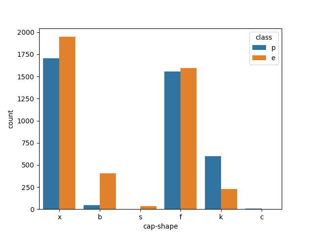
对于菌盖形状我们可以看到对是否有毒并没有很明显的区分性
- cap-color(菌盖颜色):
import pandas as pd
import matplotlib.pyplot as plt
import seaborn as sns
# 引入数据集
data = pd.read_csv(open('mushrooms.csv'))
# 绘制特征的柱状图
sns.countplot(x="cap-color", hue="class", data=data)
plt.show()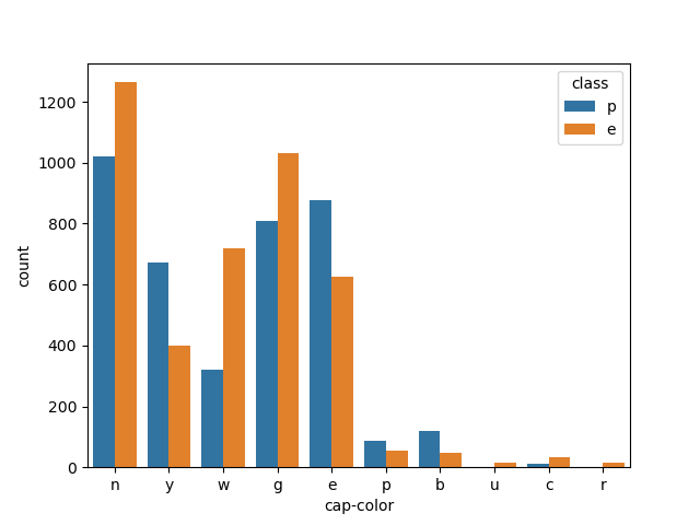
菌盖颜色的特征依然看到对是否有毒并没有很明显的区分性
- odor(气味):
import pandas as pd
import matplotlib.pyplot as plt
import seaborn as sns
# 引入数据集
data = pd.read_csv(open('mushrooms.csv'))
# 绘制特征的柱状图
sns.countplot(x="odor", hue="class", data=data)
plt.show()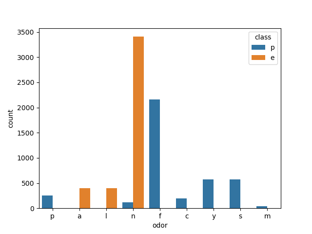
对气味属性的特征可以看到具有明显的有毒/无毒的区分度,当气味呈现焦油味=c,鱼腥味=y,恶臭味=f,辛辣味=p,辣味=s时数据集的蘑菇均为毒蘑菇,气味呈现杏仁味=a,茴香味=l时均为无毒蘑菇可食用,当蘑菇无味时,可食用无毒蘑菇占大部分,但是仍然存在少量毒蘑菇
- 从蘑菇的单个特征分析可以看出,部分属性对于蘑菇是否有毒具有强关联性,为了进一步判断蘑菇的各项特征与是否有毒之间的关联性强弱,我选取了卡方检验(chi-squared test)指标对于蘑菇数据集进行进一步的研究
2、卡方检验判断关联性
- 特征是用于训练模型的输入变量,它们是用来描述蘑菇的各种属性。在蘑菇数据集中,特征包括蘑菇的各种属性,如帽形状、帽表面的光滑度、蘑菇的气味等。
卡方检验方法:
卡方检验的p值用于判断两个变量之间是否存在显著的关联性。在蘑菇数据集的上下文中,使用卡方检验来判断某个蘑菇特征(比如
cap-shape)与蘑菇是否有毒的关联性。接下来将对所有属性特征进行卡方检验判断关联性
import pandas as pd
from scipy.stats import chi2_contingency

# 数据集路径
data_path = "mushrooms.csv"

# 读取数据集
df = pd.read_csv(data_path)

# 选择所有特征进行卡方检验
features_to_analyze = df.columns[1:]  # 排除目标变量 'class'

for feature_to_analyze in features_to_analyze:
    # 创建一个列联表
    contingency_table = pd.crosstab(df[feature_to_analyze], df['class'])

    # 执行卡方检验
    chi2, p, _, _ = chi2_contingency(contingency_table)

    # 输出卡方检验结果
    print(f"Chi-squared test for {feature_to_analyze} and class:")
    print(f"Chi2 Value: {chi2}")
    print(f"P-Value: {p}")
    print("")
输出结果:
Chi-squared test for cap-shape and class:
Chi2 Value: 489.91995361895573
P-Value: 1.196456568593578e-103
Chi-squared test for cap-surface and class:
Chi2 Value: 315.0428312080377
P-Value: 5.518427038649143e-68
Chi-squared test for cap-color and class:
Chi2 Value: 387.59776897722986
P-Value: 6.055814598336574e-78
Chi-squared test for bruises and class:
Chi2 Value: 2041.4156474619554
P-Value: 0.0
Chi-squared test for odor and class:
Chi2 Value: 7659.726740165339
P-Value: 0.0
Chi-squared test for gill-attachment and class:
Chi2 Value: 133.9861812865668
P-Value: 5.501707411861009e-31
Chi-squared test for gill-spacing and class:
Chi2 Value: 984.1433330144739
P-Value: 5.0229776137324786e-216
Chi-squared test for gill-size and class:
Chi2 Value: 2366.8342569059605
P-Value: 0.0
Chi-squared test for gill-color and class:
Chi2 Value: 3765.7140862414803
P-Value: 0.0
Chi-squared test for stalk-shape and class:
Chi2 Value: 84.14203826548719
P-Value: 4.604746212155192e-20
Chi-squared test for stalk-root and class:
Chi2 Value: 1344.4405265497817
P-Value: 7.702047904943513e-290
Chi-squared test for stalk-surface-above-ring and class:
Chi2 Value: 2808.2862874186076
P-Value: 0.0
Chi-squared test for stalk-surface-below-ring and class:
Chi2 Value: 2684.4740763290574
P-Value: 0.0
Chi-squared test for stalk-color-above-ring and class:
Chi2 Value: 2237.898496448818
P-Value: 0.0
Chi-squared test for stalk-color-below-ring and class:
Chi2 Value: 2152.390890598281
P-Value: 0.0
Chi-squared test for veil-type and class:
Chi2 Value: 0.0
P-Value: 1.0
Chi-squared test for veil-color and class:
Chi2 Value: 191.22370152470322
P-Value: 3.320972749169678e-41
Chi-squared test for ring-number and class:
Chi2 Value: 374.7368308267115
P-Value: 4.23575764172306e-82
Chi-squared test for ring-type and class:
Chi2 Value: 2956.6192780575316
P-Value: 0.0
Chi-squared test for spore-print-color and class:
Chi2 Value: 4602.0331700846045
P-Value: 0.0
Chi-squared test for population and class:
Chi2 Value: 1929.740890902809
P-Value: 0.0
Chi-squared test for habitat and class:
Chi2 Value: 1573.777260825262
P-Value: 0.0- 对卡方检验结果进行可视化
import pandas as pd
import seaborn as sns
import matplotlib.pyplot as plt
from scipy.stats import chi2_contingency

# 数据集路径
data_path = "mushrooms.csv"

# 读取数据集
df = pd.read_csv(data_path)

# 选择所有特征进行卡方检验
features_to_analyze = df.columns[1:]  # 排除目标变量 'class'

# 存储结果的列表
p_values = []

# 遍历每个特征进行卡方检验
for feature_to_analyze in features_to_analyze:
    # 创建一个列联表
    contingency_table = pd.crosstab(df[feature_to_analyze], df['class'])

    # 执行卡方检验
    _, p, _, _ = chi2_contingency(contingency_table)

    # 将p-value存储到列表中
    p_values.append(p)

# 创建一个DataFrame,将特征和对应的p-value存储起来
p_values_df = pd.DataFrame({'Feature': features_to_analyze, 'P-Value': p_values})

# 排序DataFrame以便于可视化
p_values_df = p_values_df.sort_values(by='P-Value')

# 绘制p-value的条形图
plt.figure(figsize=(10, 8))
sns.barplot(x='P-Value', y='Feature', data=p_values_df, palette='viridis')
plt.title('P-Values for Chi-squared Test of Independence')
plt.xlabel('P-Value')
plt.ylabel('Feature')
plt.xscale('log')  # 使用对数刻度以便更好地展示小的p-value
plt.show()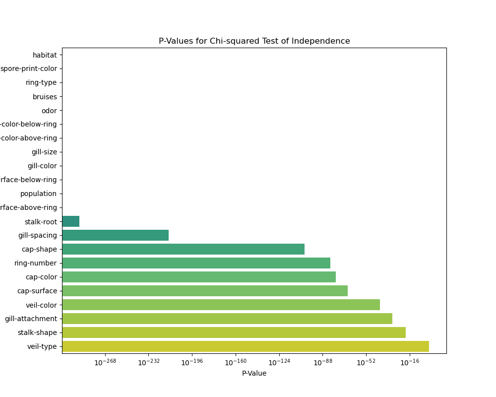
3、卡方检验结果分析
具体而言,卡方检验的步骤是比较观察到的数据与期望的数据分布之间的差异。如果差异足够大,就会导致p值很小,从而我们有足够的证据拒绝原假设,即两个变量是独立的。反之,如果p值较大,则我们没有足够的证据拒绝原假设,即两个变量可能是独立的。
在具体应用中,通常会设定一个显著性水平(通常是0.05),如果p值小于这个水平,我们就拒绝原假设。这意味着我们有足够的证据认为两个变量之间存在关联性。
总结一下:
- p值小于显著性水平(通常是0.05): 我们有足够的证据拒绝原假设,认为两个变量之间存在显著关联。
- p值大于显著性水平: 我们没有足够的证据拒绝原假设,不能确定两个变量之间是否存在显著关联。
在蘑菇数据集中,如果对某个特征执行卡方检验的p值很小,就意味着这个特征可能与蘑菇是否有毒有显著关联。这样的特征可能对于判断蘑菇是否有毒具有重要的信息。
结论:对于数据集的p值进行分析可知:habitat、odor等特征与是否有毒具有非常强的关联性。
二、模型训练
由于该数据集比较规范并没有缺失值和异常值,因此直接进行标签编码、特征编码和数据划分。
1、数据划分
将数据划分为训练集与测试集
X = df.drop('class', axis=1)
y = df['class']
X = pd.get_dummies(X)
X_train, X_test, y_train, y_test = train_test_split(X, y, test_size=0.2, random_state=42)
2、SVM模型训练
svm_model = SVC()
svm_model.fit(X_train, y_train)
3、决策树模型训练
dt_model = DecisionTreeClassifier()
dt_model.fit(X_train, y_train)
4、朴素贝叶斯模型训练
nb_model = GaussianNB()
nb_model.fit(X_train, y_train)
5、SVM模型评估
svm_pred = svm_model.predict(X_test)
svm_accuracy = accuracy_score(y_test, svm_pred)
svm_conf_matrix = confusion_matrix(y_test, svm_pred)
svm_classification_report = classification_report(y_test, svm_pred)
6、决策树模型评估
dt_pred = dt_model.predict(X_test)
dt_accuracy = accuracy_score(y_test, dt_pred)
dt_conf_matrix = confusion_matrix(y_test, dt_pred)
dt_classification_report = classification_report(y_test, dt_pred)
7、朴素贝叶斯模型评估
nb_pred = nb_model.predict(X_test)
nb_accuracy = accuracy_score(y_test, nb_pred)
nb_conf_matrix = confusion_matrix(y_test, nb_pred)
nb_classification_report = classification_report(y_test, nb_pred)
8、SVM模型结果
SVM Accuracy: 1.0
SVM Confusion Matrix:
 [[843   0]
 [  0 782]]
SVM Classification Report:
               precision    recall  f1-score   support
           e       1.00      1.00      1.00       843
           p       1.00      1.00      1.00       782
    accuracy                           1.00      1625
   macro avg       1.00      1.00      1.00      1625
weighted avg       1.00      1.00      1.00      1625
9、决策树模型结果
Decision Tree Accuracy: 1.0
Decision Tree Confusion Matrix:
 [[843   0]
 [  0 782]]
Decision Tree Classification Report:
               precision    recall  f1-score   support
           e       1.00      1.00      1.00       843
           p       1.00      1.00      1.00       782
    accuracy                           1.00      1625
   macro avg       1.00      1.00      1.00      1625
weighted avg       1.00      1.00      1.00      1625
10、朴素贝叶斯模型结果
Naive Bayes Accuracy: 0.96
Naive Bayes Confusion Matrix:
 [[778  65]
 [  0 782]]
Naive Bayes Classification Report:
               precision    recall  f1-score   support
           e       1.00      0.92      0.96       843
           p       0.92      1.00      0.96       782
    accuracy                           0.96      1625
   macro avg       0.96      0.96      0.96      1625
weighted avg       0.96      0.96      0.96      1625
三、结果分析
该模型中训练集为80%,测试集为20%
SVM 模型
- 准确度 (Accuracy): 1.0,即100%。模型在测试集上完全正确分类。
- 混淆矩阵 (Confusion Matrix): 所有的真正例(True Positive)和真负例(True Negative)都为 0,说明没有任何分类错误。
- 分类报告 (Classification Report): Precision、Recall 和 F1-Score 都是 1.0,对于每个类别都取得了最高的性能。
决策树模型
- 准确度 (Accuracy): 1.0,即100%。模型在测试集上完全正确分类。
- 混淆矩阵 (Confusion Matrix): 所有的真正例(True Positive)和真负例(True Negative)都为 0,说明没有任何分类错误。
- 分类报告 (Classification Report): Precision、Recall 和 F1-Score 都是 1.0,对于每个类别都取得了最高的性能。
朴素贝叶斯模型
- 准确度 (Accuracy): 0.96,即96%。模型在测试集上的整体准确度较高,但略低于SVM和决策树。
- 混淆矩阵 (Confusion Matrix): 有一些假正例 (False Positive),造成 Precision 和 Recall 略低。
- 分类报告 (Classification Report): 对于有毒蘑菇('p'类),Precision 较低,可能存在一些误判。Recall 和 F1-Score 对于无毒蘑菇('e'类)较高。
在该项目中,通过使用机器学习的方法来解决蘑菇分类的问题。对蘑菇数据集的22个属性特征进行可视化分析、相关性分析,使用SVM、决策树、朴素贝叶斯三种算法对蘑菇是否有毒的分类任务进行训练和测试,得到的模型准确度均达到100%,可以认为达到了预期的分类效果。
